Lab 5
Quick Stats
Time Spent: 14 Hours, I stopped counting minutes and seconds
Timers Initialized: 2 - 1 = 1
Consistent Surprise (you’ll see): 22%
CMSIS: Used Effectively
Times I Asked Xavier to Borrow the Tachometer: 1 (he just let me have it)
Individual Tachometer Measurements: >100 (thanks Xavier!)
DC Motors in the Lab: Too Hard to Find
Overall: Success
Lab 5: Interrupts
Lab Task: Read in a Motor’s Encoder for RPM
In this lab, students were tasked with obtaining the rotational speed of a DC motor using a built-in encoder. After determining this speed, students printed it out to the user in a method of their choosing.
Understanding the Hardware
I was completely unfamiliar with quadrature encoders before this lab, but have rapidly come to recognize their utility. Professor Joshua Brake created the following animation, in Figure 1, to describe their behavior. It can be found in the prompt for Lab 5 here. I found it to be the most effective tool for gaining an understanding.
This diagram shows the waveforms generated by our DC motor’s encoder, which consists of two lines: an A and a B. Using just these offset waveforms, one can determine both the rotational speed and direction of the motor. Finding the speed is easy – it’s directly linked to the frequency of the wave. In Figure 1, a single rotation contains 6 dark and 6 light sectors, generating 6 rising edges and 6 falling edges on the waveforms A and B. By counting the time between edges, whether one counts between two or waits for a full cycle of twelve, one can manipulate this value to determine the revolutions per second of the motor. Alternatively, by counting the amount of edges in a given amount of time, one can similarly determine the motor’s rotational velocity.
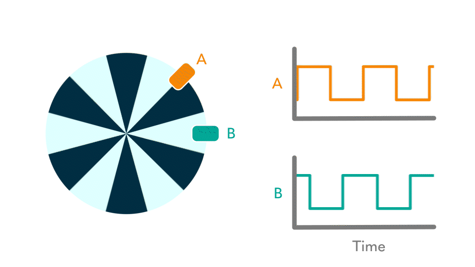
The direction, on the other hand, is less straightforward. It may not be immediately obvious how one can track the direction just from these alternating waveforms. The key idea is that the offset between the two waves generates a unique pattern which depends on the direction of spin. This is easiest for me to visualize if I track a single trough on the lower B waveform. You’ll notice that within the bounds of one of these low B troughs, the A wave is low on the left portion and high on the right. Focus in on the left portion of the trough – here, the B wave is low and the A wave is low. Track one of these points of low-low. Imagine that the motor came to a standstill on one of these points, and the animation stopped moving. If you were looking from within this low-low trough, you would see an B waveform high to the left, and an A waveform high to the right. Either direction you spin the motor, you would run into one, and only one, of these rising edges first. This is how one can track motor direction.
Put another way, the encoder’s current state is listed like a coordinate pair, {AB}, where a low-low trough is represented as {00}. No matter the current state, whether it be {00}, {01}, {10}, or {11}, there are only two possible next states. Each possibility corresponds to a different direction.
Great! So, if we track the timing of the waveform edges, we get rotational velocity – if we track the state of each wave, we get motor direction. How do we translate this into C code which we can implement on a microcontroller (MCU)?
Introducing: Interrupts
Fundamentally, the question is how best to track these edge changes. There are two broad categories which describe the two different fundamental implementations – a solution either uses interrupts or polling. Polling is the easier to implement. One could track the edges by “looking” at the signal at a set interval. For example, one could check the status of the encoder every 10 milliseconds, thus constructing a discrete graph of the signal over time. This is much like we programmed into our Lab 3 keyboard scanner, which checked every row of the keypad for a millisecond. Detection was not instantaneous – it relied on a polling time that was fast enough to pick up inputs “as if” in real time.
Interrupts, on the other hand, are more difficult to implement on an MCU. However, they can be more useful when a precise response to real-time inputs is required. Instead of relying on the central processing unit (CPU) to track a timer and poll the input, a dedicated peripheral watches for changes. This peripheral then reports changes to the CPU, which temporarily pauses its main task to handle the generated “interrupt” before returning to its previous function. In this way, one can track the status of a wave as it changes in real time, while at the same time leaving the CPU to handle other tasks along the way.
When choosing between the two, I should first state that I always planned to use interrupts for this lab – after all, that was a core learning goal. However, I believe that it represents the better choice in this case because it is the only way to construct a full, non-discrete image of the waveform. I use non-discrete loosely here, because we are still limited to checking for an interrupt on every CPU clock cycle, but the key point is that we can track changes with for more accuracy than we could in a polling system. By only checking for changes in the system, we can construct a much fuller picture while reducing CPU overhead. Note, however, that there is a limit. We can only log our edges as fast as our CPU can process interrupts. This case happens to work well, since I calculate that we might generate up to 5000 interrupts a second, leaving >3,500 clock cycles between interrupts. If we were to generate a million interrupts a second, on the other hand, then my interrupt-handling code is likely too long to keep up. My printing code in the main loop would never run, and I would under-count generated edges. This could be partially fixed by interrupt-proofing my print loop, or by making the timer generate a higher priority interrupt to print, but neither of these measures were necessary for my relatively slow case. Additionally, interrupts work well here because I am only expecting one signal to change at any one time. I would need to fundamentally redesign my system if I was expecting a sudden influx of signals changing in parallel, since each interrupt change would be backlogged behind another. However, if I was truly getting into sub-microsecond changes and logging multiple parallel signals, I would likely choose to use an FPGA anyways.
Microcontroller Block Diagram and Schematic
To implement an interrupt-based system on my MCU, I first had to choose how I planned to measure my system. Initially, I supposed that timing the difference between pulses might offer the best way to determine my motor’s speed. However, after this idea ended up producing significant error (up to 25%!), I instead pivoted to measuring the amount of pulses in a longer, fixed time. In order to measure direction, I stuck to the stage-based system which I previously discussed.
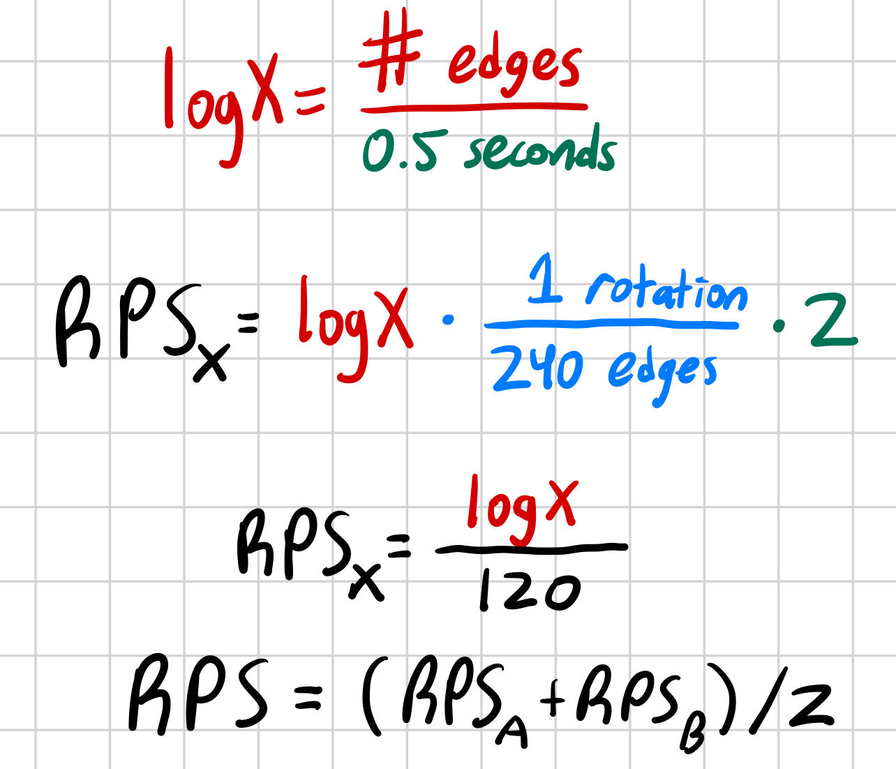
To turn this into code, I chose to create a main loop which contained a frame timer and my printing logic. This main loop was responsible for initiating and waiting for a half second timer, calculating revolutions per second (RPS), and printing to the user. In order to calculate RPS, I could create global variable logA and logB. Each time an edge came, I could increment the related logX variable. So, by manipulating the logX variable according to the equations in Figure 2, I could prepare them for the print statement. Speaking of, the print statement was relatively straightforward. By leaving the SEGGER debugger attached to the MCU via microUSB, we could print to it at our whim. I followed a tutorial created by Kavi Dey, found on a website of his here. You can find out more about my implementation by looking at my Github code, in the source > lib folder titled DEBUG.
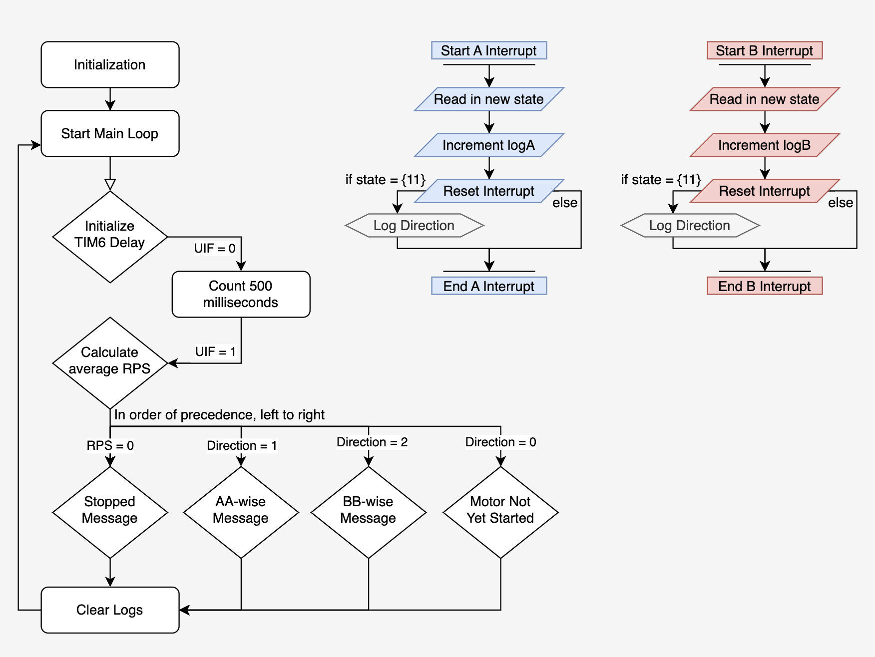
Then, in order to track direction and actually log the pulses, I made use of interrupts. In the MCU, we can use logic contained within a GPIO pin block to monitor a signal, generating a unique interrupt for each A and B signal. By setting this interrupt to occur on each rising and falling edge and logging the respective logX variable, we can properly give the main function everything it needs to calculate the RPS. By tracking the state of the system at the beginning of each interrupt, then comparing it to see what direction the motor is traveling, we can thus determine direction and log that in a global variable visible to the main loop. A summary of this description may be found in the flowchart in Figure 3 below.
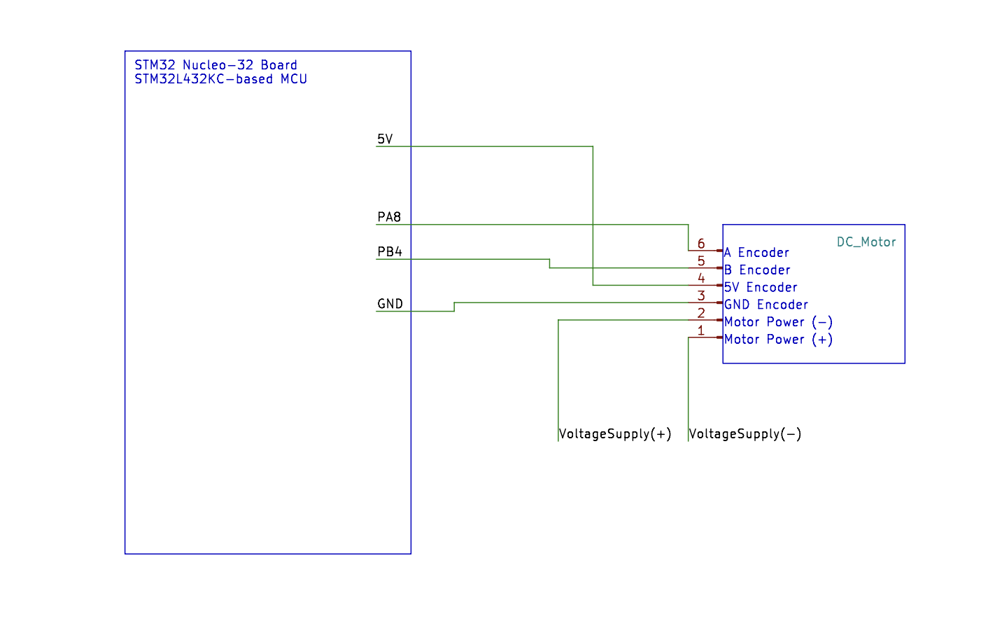
Finally, attaching this system to our MCU is straightforward. We are given a 25GA-370 DC motor, with the datasheet our class references available here. It requires a DC voltage supply between 0 and 12V, which I provided from a benchtop power supply (as seen in the system demo video above). I chose to attach the A encoder and B encoder signals to GPIO A and B ports respectively, making the code easy to parse. The simple schematic may be seen in Figure 4 below.
Testing the System
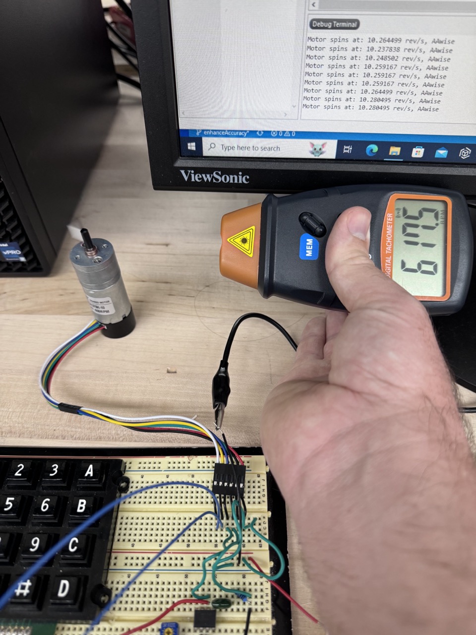
As I tested version two of this system – which counts pulses within a 500 millisecond framing window, instead of timing between pulses – I noted a constant error. My output values seemed to be near 20% lower than my actual RPS. How do I know? I measured it, using a tool called a tachometer. This handheld tool, seen working in the video linked here, uses a laser and reflective tape to accurately calculate the RPM of a mechanical system. Using this, I was able to generate the table in Figure 5, describing my MCU captured values against my Tachometer values.
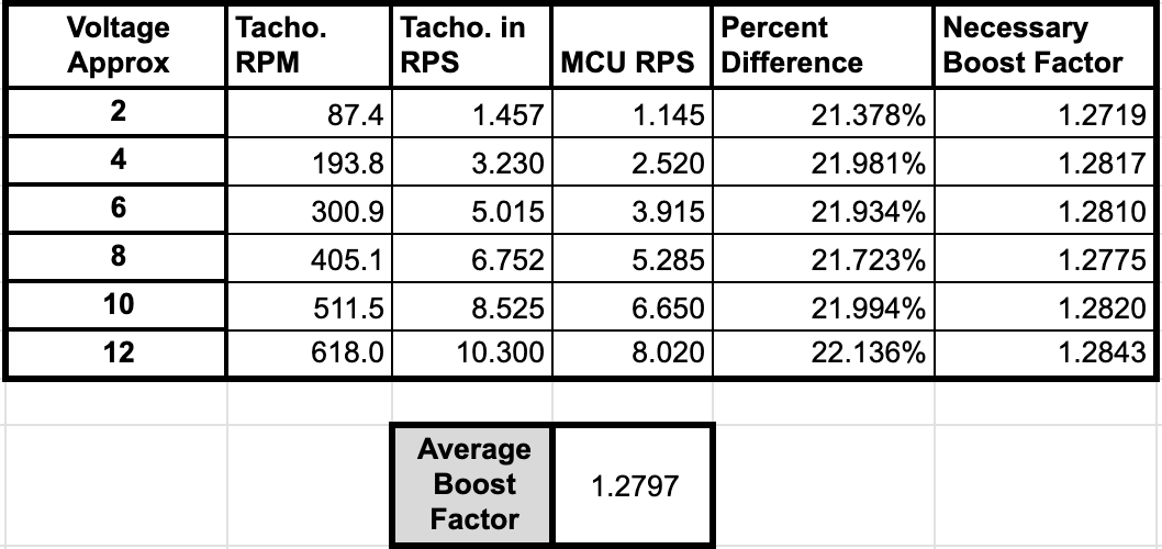
This table shows a consistent error, where my output value is between 21.1 and 22 percent lower than the actual value, assumed as equal to the tachometer. This consistent error is confusing to me. The first place I checked was my frame timer – if this was shorter than anticipated, then it would be under-reporting the true RPS. However, after counting a sequence of 60 cycles, I found that it was in fact under-reporting… by 1.06%. This is nearly within the error on the system clock itself, and certainly not significant enough to describe the consistent error. I then wondered if I could somehow be going too fast, and missing interrupts. However, the consistency of my error across voltages made me consider this a poor explanation. If this were the case, then I would have expected the error to grow with voltage as the system missed a larger and larger portion of the available pulses. Even now, I see no reason for this 22% error. It is not a simple factor of two error, nor could I imagine how it might come from my calculations. If only my B encoder counted at half the rate, then this could lead to a close ~25% drop. However, I checked both my A and B counters separately and they both had the same independent error. So, I do not know the source of this error.
However, I do know how to fix it. Since it is a constant error, applying a simple multiplication factor does the trick. However, I felt that it would be simplest to add this value in as an integer. To do so, I decided to add in a topFactor and botFactor integer to my code, effectively scaling my answer by (topFactor/botFactor). The closest integers I could find under 1000 were topFactor = 947 and botFactor = 740. Using these integer values introduces an error of <0.05%. After implementing this scalar, my printed RPS values were extraordinarily spot on. As seen in Figure 6, I was able to measure in a velocity with an error below 1%, sometimes approaching nearly 0.1%. I am quite pleased with these results, even if I am unable to locate the mysterious 22% error.
Watch the Tachometer video here!! Youtube wouldn’t let me embed it here since I filmed vertically.
Finally, I want to mention that the system correctly reads out the direction, recognizing a clockwise, counterclockwise, and stopped motor.